# Report Claims DeepSeek-V4-Flash Initialized on Export-Controlled NVIDIA GPUs: Three Paths of AI Hardware Side Channels
Published: 2026-11-18 · Language: en
Original: https://yage.ai/share/gpu-side-channel-forensics-en-20261118.html
Publisher: Superlinear Academy · 100% AI generated
[Article index](https://yage.ai/share/llms.txt)
[Other language](https://yage.ai/share/gpu-side-channel-forensics-20261118.html)
In mid-November, [Unemployment Labs published a report](https://unemploymentlabs.com/checkpoint-forensics) showing that solely by analyzing publicly downloaded model weights, they inferred that six recent Chinese frontier models—including DeepSeek-V4-Flash and Kimi K3—were initialized on NVIDIA Blackwell GPUs subject to U.S. export controls. Because this generation of chips falls under export restrictions to China, the report quickly drew wide attention across the industry.
Setting aside the compliance debate, what makes this research technically compelling is its underlying forensic logic: after a model finishes training and its weight files are publicly released, how can traces of the specific GPU model still remain inside the numbers? Zooming out across the model lifecycle—from initial weight generation and low-precision training to online inference serving—physical traits of the underlying hardware can leak into static weights or runtime outputs at every stage. Below, we first explain how the report reads GPU models out of weight files, and then trace the other two hardware side channels across the model lifecycle along with their current empirical maturity and mitigation costs.
## Why Do Initial GPU Traces Survive After Training Finishes?
Before training begins, PyTorch treats the entire weight matrix as a continuous strip of hundreds of millions of cells and invokes NVIDIA’s Philox algorithm to fill it with random initial values. To populate billions of parameters quickly, all Streaming Multiprocessors (SMs) on the GPU work in parallel, with each SM launching a fixed squad of 2,048 worker threads. Different GPU generations have different SM counts: the previous-generation Hopper H100 has 132 SMs, fielding roughly 270,000 worker threads at once; the newer Blackwell B200 has 148 SMs and the GB200 has 152 SMs, expanding the total crew to roughly 303,000 and 311,000 threads respectively.
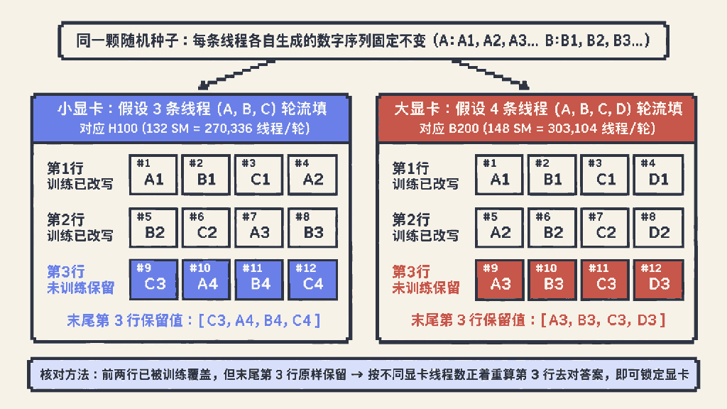
Given the same random seed, the sequence of numbers generated by each individual thread is completely fixed: regardless of which GPU is used, the thread with the same ID always produces the exact same 1st number, 2nd number, and so on. However, when writing those numbers into the weight matrix, all threads on the card take turns filling cells one by one in order of their thread IDs. The simplified 3-row by 4-column diagram below illustrates why this matters: on the left, a smaller GPU with only three threads (A, B, and C) taking turns finishes its first round in the first 3 cells, so cell \#4 immediately receives thread A’s second-round value; continuing down the grid, the bottom row ends up holding `C3, A4, B4, C4`. On the right, switching to a larger GPU adds a fourth thread D, so four threads take turns and each 4-cell row neatly completes one round, leaving `A3, B3, C3, D3` in the bottom row.
Even though the random seed is identical and every thread generates the exact same personal sequence of numbers, simply changing the total number of threads taking turns alters the stride of every round, shifting subsequent rows further and further apart. In a real model spanning hundreds of millions of cells, the values written into the same row by an H100 versus a B200 come from completely different threads and rounds.
Coordinate differences when writing a weight matrix from the same random seed on H100 vs B200
Why does that bottom row survive all the way to the end of training? That comes down to how the vocabulary embedding matrix is updated. While parameters in the middle layers of a neural network are updated all together on every training sentence, the opening vocabulary matrix works like an indexed lookup table: only the single row corresponding to a word that actually appears in the training text gets updated, whereas any row whose word never appears stays completely untouched. In real large language models, there is always a batch of rows that never appear once during pre-training: some are rare symbols that never show up in the corpus or reserved special tokens set aside for later post-training chat stages, while others are hundreds of padding rows appended at the end of the vocabulary so the matrix row count rounds up to a multiple of 128. The numbers in these rows are never modified by gradient updates and preserve their exact initialization state; moreover, their exact row indices and cell offsets are directly visible as soon as you open the publicly downloaded weight file.
Because the exact position of these untouched tail rows is known, external researchers do not need to reverse-engineer a scrambled permutation; they simply compute forward to check the answer. By assuming a candidate random seed and simulating the round-robin rules of an H100 versus a B200, researchers directly calculate which numbers should land in those untouched tail rows and compare them against the downloaded weight file. Because PyTorch’s default 32-bit random seed has only about 4.3 billion possibilities, the research team brute-forced all possible seeds across common GPU thread counts, checking roughly 6 trillion combinations in total. Whenever the seed or GPU model is wrong, the locally computed numbers show zero correlation with the untouched row in the file; once both match, all several thousand numbers in the row align element by element with a correlation coefficient exceeding 0.999.
Using this method, the team matched Blackwell layouts in six recent Chinese models including DeepSeek-V4-Flash, Kimi K3, and MiniMax-M3, whereas earlier releases such as DeepSeek-V3 and contemporaneous models like GLM-5 matched the previous-generation Hopper layout. To verify their findings, the team rented physical H100 and GB200 GPUs and reproduced the exact untouched rows of DeepSeek-V3 and Kimi K3 on real hardware. They also checked the compute-unit layout of AMD’s MI300X GPU, confirming that all distinguishing points in DeepSeek-V4-Flash pointed exclusively to NVIDIA, and open-sourced their entire [reproduction codebase](https://github.com/macrogrants/checkpoint-forensics).
One day later, developer Bojie Li published an [independent reproduction report](https://01.me/2026/11/checkpoint-forensics/) and an [extended scanning toolkit](https://github.com/bojieli/checkpoint-forensics). Scanning more than two hundred open-weight models, he identified 185 hardware thread-count fingerprints covering both Chinese models and overseas releases such as NVIDIA Nemotron.
What if a vocabulary table leaves no completely untouched rows? Traces can still survive. In Xiaomi’s MiMo-V2.5-Pro-Base, every row in the vocabulary participated in training, so each final weight equals its initial random value plus accumulated training updates. Because training updates are much larger than initial values, comparing any single row against the initial sequence yields a negligible median similarity of just 0.034; yet when more than ten thousand rows are aggregated together, training updates for different words point in varied directions and cancel out statistically, allowing the true initial sequence to contribute a consistent positive alignment across every row and surfacing the Hopper layout clearly. Another common case occurs when training enables weight decay: at every step, the optimizer multiplies all parameters by a positive factor slightly smaller than one, shrinking values toward zero. In Qwen2-7B, unused vocabulary rows shrank all the way down to the smallest non-zero value representable by the storage format, leaving every number with the exact same magnitude; however, because multiplying by a positive factor never flips a sign, the sequence of plus and minus signs across the entire row still matches the Hopper initial sequence 100%.
Still, this method has clear technical boundaries. It only identifies the hardware thread specification at the exact moment initial weights were generated, and any two GPU models with the same SM count share the same total thread count and cannot be distinguished by layout alone. As for whether subsequent full-scale training remained on the same class of GPUs throughout, static weights alone cannot provide direct proof, since checkpoints can be saved to disk and moved to a different cluster at any point.
## If Switching to CPU Initialization Erases That Trace, Do Static Weights Hold Other Clues?
Although initialization fingerprints are precise, erasing them is straightforward. Among the models scanned by Bojie Li, dozens yielded no GPU fingerprint: some generated initial weights sequentially on a CPU, some overwrote unused vocabulary rows with CPU random numbers after training finished, and others like DeepSeek-V4.1-Flash retained seemingly untouched rows that matched no known GPU layout or seed, likely due to modified initialization code. Simply bypassing default GPU parallel initialization breaks this first trail completely.
If initialization is moved to the CPU, do trained weights still retain arithmetic traces of the training GPUs? In theory, another clue lies in how low-precision training groups weights for scaling. To save memory and boost throughput, large model training increasingly compresses high-precision parameters into 8-bit or even 4-bit low-precision formats. Once the bit width is reduced, a 4-bit value—excluding its sign—can only represent a handful of discrete ticks such as 0.5, 1, 1.5, 2, 3, 4, and 6. To fit real weights spanning a wide dynamic range into those few ticks, adjacent weights must be grouped into small blocks that share a common scaling multiplier, representing every number in the block as that shared multiplier times one of the fixed ticks. According to [NVIDIA’s technical documentation](https://developer.nvidia.com/blog/introducing-nvfp4-for-efficient-and-accurate-low-precision-inference/), Hopper’s primary 8-bit format typically shares a scaling multiplier across hundreds of parameters or an entire matrix, whereas Blackwell’s native 4-bit format hardware-enforces a separate scaling multiplier for every 16 adjacent parameters.
Why could this hardware format difference leave a trace? Within a single 16-parameter block, every number is produced by multiplying the same shared factor against those few fixed ticks, locking their mutual ratios onto a single grid; stepping into the 17th parameter starts a new block with a different multiplier. In principle, testing whether scaling grids reset every 16 elements along a weight matrix could reveal whether training ran on Blackwell’s native low-precision hardware pipeline. In practice, however, this path remains at the stage of theoretical inference: pre-trained models typically undergo high-precision supervised fine-tuning and reinforcement learning before being repackaged into standard formats for release, and those continuous parameter updates blur the 16-element grid boundaries. No open-source tool capable of reliably extracting this signal across large sets of models exists yet.
## When Only an Online API Is Exposed, Can External Probes Identify the Inference GPUs?
Both static approaches require access to downloaded weight files and examine what hardware was used before release. What if a model is already deployed behind a black-box chat API that hides its server GPUs, inference software stack, and quantization settings? Here, testing strategies split into two paths depending on whether the underlying model weights are open-source.
The first path applies when a cloud provider hosts a model whose weights are publicly known. Even without backend access, the tokens emitted by the model can betray arithmetic differences in the underlying hardware. In floating-point addition, adding the first two numbers before the third versus adding the last two before the first can produce a tiny rounding difference in the last place; [Thinking Machines Lab’s engineering analysis](https://thinkingmachines.ai/blog/defeating-nondeterminism-in-llm-inference/) demonstrated that even when sampling temperature is set to zero to disable random sampling, slight shifts in parallel summation order on the server cause candidate token scores to drift in the late decimal places.
Different GPU generations and inference engines partition matrix multiplications and parallel reductions in distinct, deterministic orders. Ordinarily, a discrepancy several decimal places down does not change which candidate token ranks first; but when the top two candidate tokens have nearly tied scores, a last-place rounding difference is enough to flip the winner, altering the emitted token and compounding across subsequent autoregressive steps. The NeurIPS paper [Fingerprinting Inference Systems of Large Language Models](https://arxiv.org/abs/2605.29979) exploits this exact sensitivity: using open-source weights locally, testers pre-screen a set of boundary prompts engineered to create near-ties between the top two candidate tokens, send those prompts to the online API, and observe which token the server favors to identify the backend hardware and software stack. On the paper’s deterministic decoding benchmark at temperature 0, these boundary probes identified the underlying GPU platform, inference engine, and attention backend with 100% accuracy; even at temperature 0.3 with random sampling enabled, repeated queries still identified the GPU model and inference engine with nearly 80% average accuracy. Because blocking this side channel requires making low-level floating-point arithmetic bit-for-bit identical across disparate chips and software stacks, defending against it in production is notoriously difficult.
The second path applies to purely closed-source APIs whose weights are never released. Unable to pre-screen boundary prompts locally, external observers can still probe the physical ceiling of token generation speed. During autoregressive decoding, generating each new token requires reading the active model weights from high-bandwidth memory (HBM) into the compute units once, making token generation speed directly bottlenecked by memory bandwidth. Among standard SXM server GPUs, the previous-generation H100 delivers 3.35 TB/s of memory bandwidth, while the newer B200 jumps to 8.0 TB/s—more than double; at the same time, compressing weight precision by half cuts the bytes transferred per token in half, similarly accelerating output speed.
That trade-off also defines the limitation of black-box speed testing: when a closed-source service discloses neither its active parameter count nor its quantization scheme, faster token generation alone cannot separate a GPU with twice the memory bandwidth from a model compressed to half the bit width. What black-box latency testing actually measures is the joint performance boundary set by memory bandwidth ceilings and weight compression.
## Signal Strength and Evasion Cost Across the Three Paths
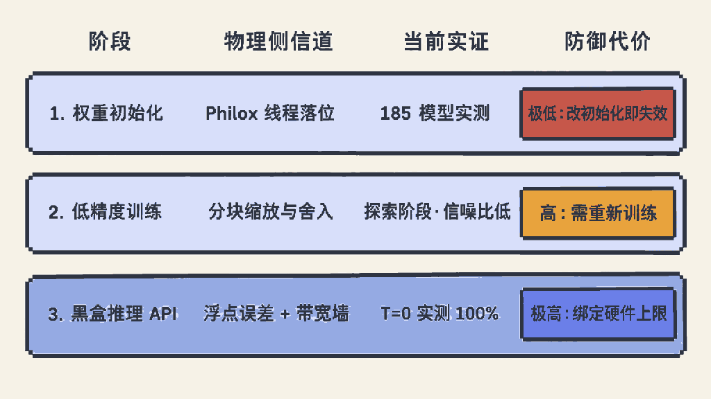
Comparison of empirical maturity and defense cost across three hardware side-channel paths in the model lifecycle
Stepping through the full lifecycle from weight initialization to online serving, the three side-channel paths show a sharp inverse relationship between empirical certainty and evasion cost. Philox initialization layouts have already been verified across 185 open-weight models and provide the sharpest static evidence today, yet they are also the cheapest to erase: switching to CPU initialization or overwriting unused vocabulary rows after training closes the leak immediately.
Low-precision block-scaling traces are tied to native GPU arithmetic formats and cannot be bypassed merely by initializing on a CPU. However, they currently remain a theoretical mechanism whose periodic grid steps are easily diluted by post-training fine-tuning and format conversion, with no large-scale cross-model detection tool available in the community.
The methods that directly confront live black-box services are inference-stage arithmetic divergence and memory-bandwidth bounds. For APIs hosting known open weights, boundary prompts that amplify floating-point summation differences have demonstrated high hardware identification accuracy in controlled benchmarks and are difficult to scrub out in engineering practice; for completely closed models, token-speed measurements cannot name a specific GPU in isolation, yet still bound the physical envelope of memory bandwidth and quantization. Software engineering relies on abstraction layers to hide underlying silicon, but under the magnifying glass of massive parallelism and low-precision arithmetic, datacenter GPUs continue to leave their physical imprint across weight matrices and API responses.