In the previous article, we used computer simulation to render a photorealistic image of the night sky. That kind of simulation gives us superpowers that real photography cannot: sky roaming, time acceleration, and simulating the Milky Way and star fields under different light pollution and visual sensitivity. In this article, we apply the same approach to the turquoise band during a total lunar eclipse.
Anyone familiar with astronomy has probably heard of it. During a total lunar eclipse, the moon is not fully black; it turns a very dark bronze color. But as the moon gradually brightens and returns to full phase, if you carefully photograph the edge of Earth's umbra, you will find that it is neither red nor white, but a layer of cyan-blue — the color of turquoise, hence the name turquoise band.
If you search for why this narrow green-blue band exists, you will usually get an answer involving the ozone layer: the light in this ring mostly comes from sunlight refracted through the ozone layer, and ozone strongly absorbs yellow-orange light, which creates the turquoise band. But if you think carefully along this line of reasoning, quite a few things do not add up. For example, why is the turquoise band so narrow? Light refracted through the ozone layer should have an angular size on the same order as the Sun, about 32 arcminutes, yet the literature gives only about 2 arcminutes. Also, if you look at the ozone absorption spectrum, its absorption of red-orange light is nearly 100 times stronger than blue-violet light, so the color should be a saturated blue-green. In practice, the turquoise band is very hard to photograph, and the blue-green color is extremely faint.
These questions made me feel that I had not really understood the underlying mechanisms. Just as in the previous article, every failure pointed to something we take for granted but had never truly understood. Why do bright stars look larger? Why does numerical simulation say we should still see the Milky Way under Class 9 light pollution, yet we cannot in reality? The gap between simulation and observation forces us to discover new knowledge.
The turquoise band is the same. In this article we will step through the simplest numerical simulation — refraction, scattering, absorption, and straight-line propagation — to actually compute the color and position of the turquoise band, and compare the results with real observations and the literature. This, too, is a journey of repeated failures, and each failure teaches us something new.
Starting from a White Disk
So we go back to the beginning. The moon is a gray-white disk with some dark maria (these textures can be downloaded from NASA). The Sun is a point source. Light hits the moon and reflects back, giving us a full moon. Nothing surprising here.
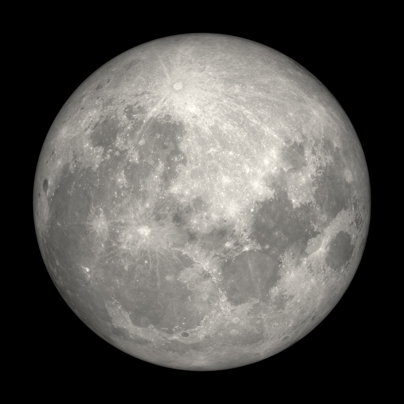
Figure 1: Starting point — a gray-white disk with lunar texture, no atmospheric physics yet
Now a lunar eclipse happens: Earth blocks the Sun and the moon. If Earth were just an opaque rock, the blocked half of the moon would be pure black, the unblocked half normal moonlight white, with a hard edge between them. That is Figure 2. (The images have simple brightness processing so they display normally on ordinary monitors; same below.)
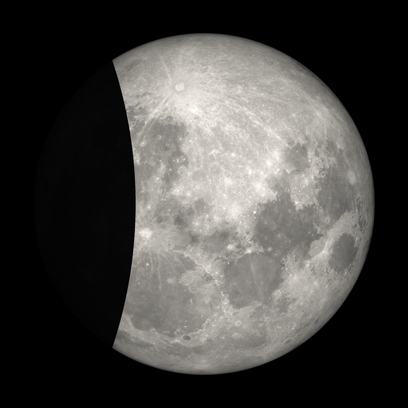
Figure 2: Geometric occlusion — half black, half white, hard edge, no atmosphere
But during a lunar eclipse the moon is not fully black, because Earth has an atmosphere. Sunlight grazing Earth's edge is refracted inward and illuminates regions that should be completely dark. This light travels tangentially through the atmosphere, so the path length through air is dozens of times longer than a vertical path. Over such a distance, light is heavily absorbed and scattered.
Here we add the most basic scattering first: Rayleigh scattering, the mechanism that makes the sky blue. Rayleigh scattering scales with the fourth power of wavelength, so blue light is scattered most strongly. When sunlight passes obliquely through dozens of times the atmospheric thickness, blue light is almost completely scattered away, leaving only red to penetrate. The dark region brightens and turns bronze-red. The blood moon appears.
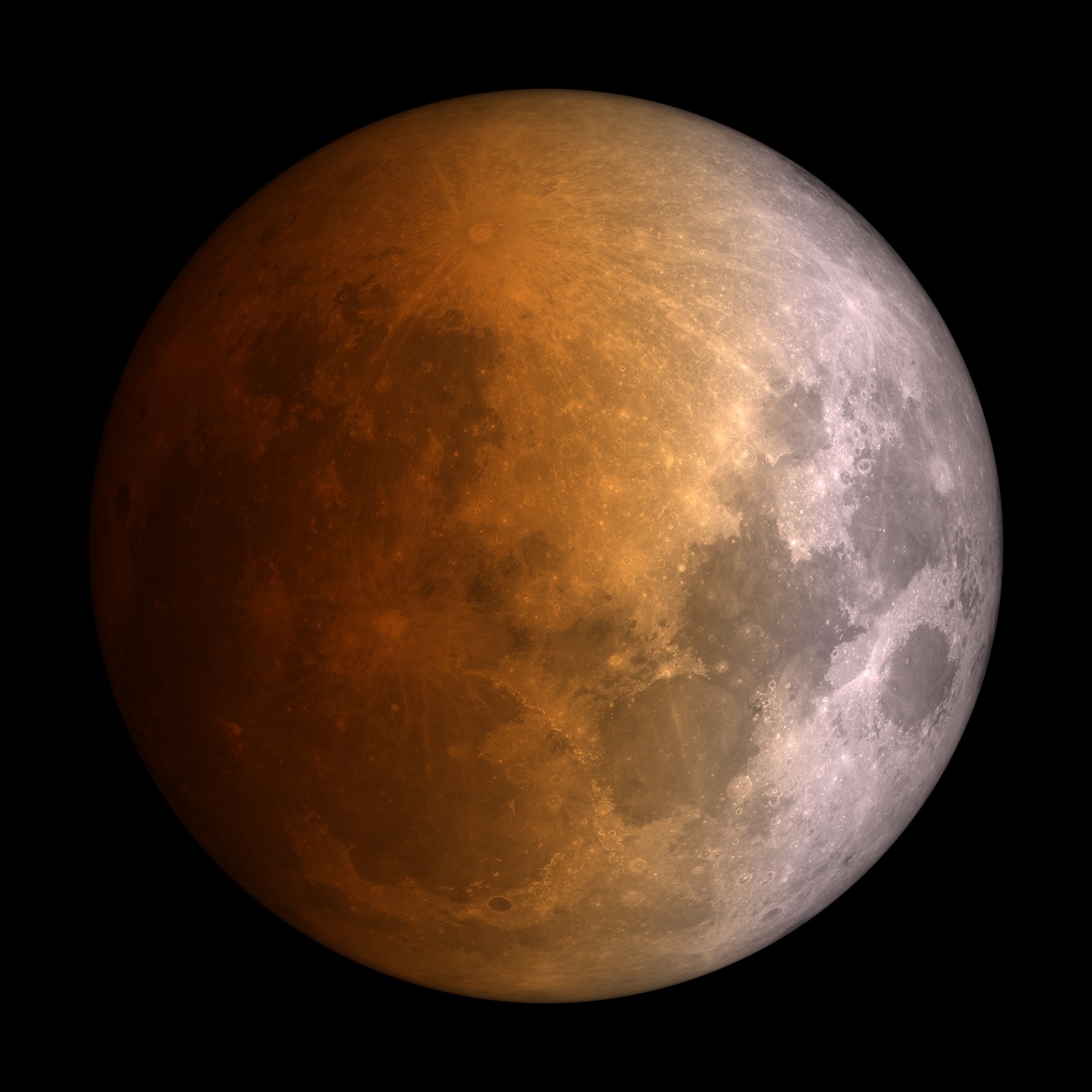
Figure 3: Rayleigh scattering added — umbra no longer fully black, blood moon red appears
Up to here everything goes smoothly; we see the familiar blood moon. Then the next step goes wrong. We add ozone absorption. Ozone has an absorption band called the Chappuis band, roughly 500 to 700 nanometers, which eats orange-red light. After adding this band, green-blue really appears, and just as the literature and intuition would predict, it is a very strong cyan band (Figure 4). The red-to-blue ratio reaches 0.53 — dazzlingly cyan.
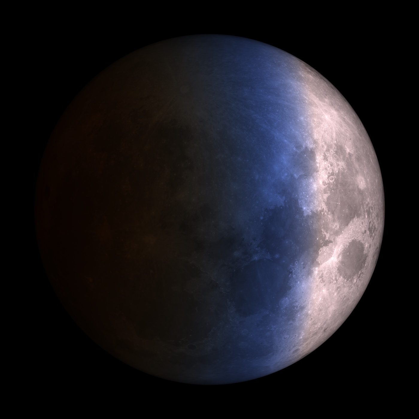
Figure 4: Chappuis ozone absorption added — cyan band appears, but much stronger and wider than reality
The problem is that this band is too strong. In real lunar eclipse photos, the turquoise band is a faint, narrow thread visible only with HDR and heavy post-processing. Such an obvious blue stripe looks fake at a glance; something must be wrong. Yet our calculation seems to miss nothing in physics: we have scattering, refraction, and ozone absorption, but the result still does not match real observation.
Where the Approximations Hide
I was stuck here for a long time. I checked the code and the data repeatedly and found nothing wrong. Eventually I realized the problem was not in the physics, but in an approximation I had not even recognized as an approximation: we treated the Sun as a point source.
The real Sun is a disk 32 arcminutes across, not a point at infinite distance. When we treat the Sun as a point source, each point on the lunar surface is lit by a single ray, corresponding to one definite grazing height. When that height falls near the ozone layer, the result is vivid blue. But in reality, different points on the solar disk send light that grazes Earth's atmosphere at different heights. Light reaching the same point on the moon comes from a bundle of rays at different grazing heights — some from the ozone layer, but most not.
The standard academic approach is to derive formulas with a point-source approximation first, then add a geometric correction at the end. For example, Mallama's 2022 review of lunar eclipse modeling uses a "for a point source of light" assumption to derive the full refraction formulas, then adds geometric corrections such as blurring. I adapted that approach to our scenario, but the results never worked (umbra brightness did not match observation).
In the end I gave up and returned to the brute-force approach from the previous article: no formula derivation, no geometric correction, but a full multi-dimensional integral over all points on the solar disk. Take many, many points, simulate many rays from each, trace each ray with refraction, scattering, and absorption, and finally see the true brightness and color. This integral immediately diluted that strong cyan band: the bluest point from the point-source calculation had a red-to-blue ratio of 0.53; after adding the solar disk it became 0.71. The cyan faded, the band widened and softened, and its position shifted inward. This is what a real lunar eclipse looks like.
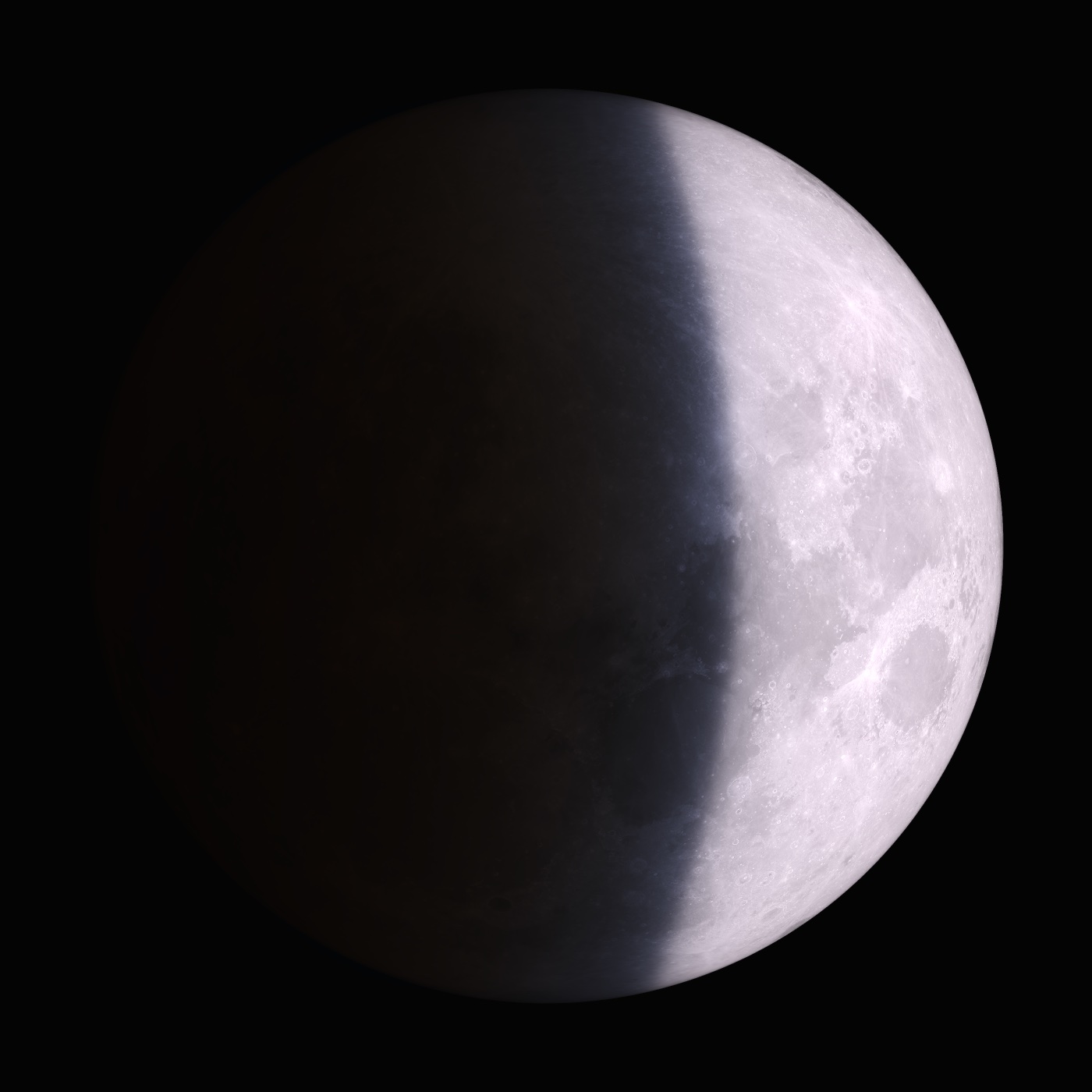
Figure 5: Solar disk added — strong cyan smeared into soft pale cyan, close to real observation
This raises a bigger question. Scientific computing in astrophysics has, for decades, developed a working style I call "the art of approximation." A phenomenon is too hard to solve, so take a first-order expansion and keep only the first two terms. Something diverges, add a correction term. That correction introduces new bias somewhere else, so add another layer. Each approximation requires deep physical intuition and hard-won experience to stay simple, fast, and correct. When supercomputer time was billed by the hour and a PhD's time cost more than compute, this was a very rational strategy. Being good at approximation was a real skill back then.
But approximation has a hidden cost: each one introduces a free parameter, and those parameters fight each other. One approximation diverges somewhere; add a patch. The patch causes bias elsewhere; add another layer. In the end you cannot tell whether error comes from physics or from the interaction of several approximations. We hit exactly this trap in the lunar eclipse project. We used four or five related approximations, each with a citation in the literature and each looking reasonable on its own. Stacked together, the brightness at the center of the umbra came out 6 stops — 250 times — brighter than reality. It is very hard to locate which layer caused the bias, because they are entangled.
Wrestling with AI
Before the AI era, I would have stopped here. I am neither strong in physics nor in computation. I do not have that kind of physical intuition. A year ago I also tried to use AI for this kind of problem and failed for the same reason: too many physical decisions, and at each decision point I had to understand why predecessors approximated the way they did, under what conditions the approximation holds, and what happens if you remove it. AI would give me code, but I could not even see where the approximations were hiding.
This year I suddenly realized: if AI is writing the code anyway, why keep all these approximations? Why not start from raw ray tracing and honestly loop over every pixel on the Sun, every height layer in the atmosphere, every wavelength in the spectrum, and every distance to the center of the umbra? Send out many rays, let them refract, absorb, scatter, and converge on their own — no clever shortcuts, just brute force. The underlying physics stays clear and simple, so the chance of error is much smaller. And turning this into performant code, say GPU kernels, is something AI is very good at. Run once on CPU, once on GPU; if the results match, the implementation is almost certainly correct and easy to verify.
So why did I still make many mistakes? Mainly because AI knows physics too well. After literature review it reflexively follows predecessors' footsteps and applies physical intuition through approximations — and leads me into traps again. Most of my time went into wrestling with AI, discovering one hidden physical approximation after another, and finally rewriting everything into the simplest, most brute-force version.
In this project, the last cut was removing an approximate focusing factor entirely. Focusing means that rays grazing Earth's edge, refracted inward by the atmosphere, converge inside the umbra and make the center brighter than the edge. The literature approximates this with an analytic 1/r formula and a hard r_floor floor to patch its infinite divergence at the center. We used that formula at first. But focusing is a natural outcome of ray tracing: scatter enough rays, let each refract to its landing point, and the density of landing points is the brightness — no formula needed. Using a formula means replacing statistical emergence with a hand-built closed form, so the umbra center came out too bright. Remove the focusing formula and use pure ray landing bins instead, and the center drops from −7.7 stops to −13.1 stops — already in the same order of magnitude as real deep totality at −14 to −19 stops. The remaining gap is aerosols and clouds in the real atmosphere, not a numerical problem.
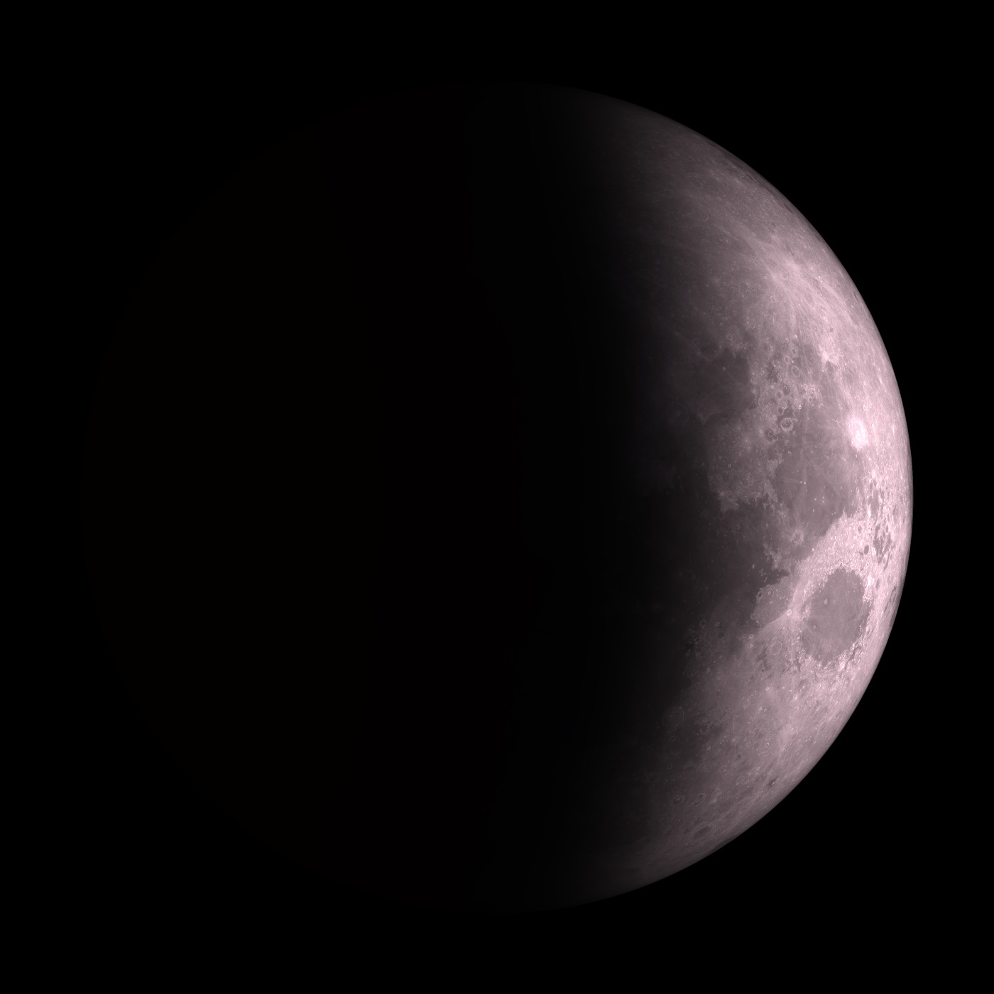
Figure 6: True forward ray tracing — focusing, landing points, and brightness all emerge from scattered rays, zero analytic prescriptions
Answers to Two Counterintuitive Questions
At this point, let us return to the two questions from the beginning.
Why is the turquoise band a narrow strip rather than a broad patch? The answer lies in brightness, not color. The color (red-to-blue ratio) varies smoothly across the lunar disk over more than ten arcminutes, with no sharp jump. But the bluest segment is also the darkest on the entire curve — only 4.5% as bright as the brightest part of the disk, too faint for the eye to see clearly. Right beside it is the normal moonlight region outside the umbra, 250 times brighter; intense white moonlight completely swamps the cyan-blue. The turquoise band we see must be neither too dark nor too bright, and blue enough — visually it is squeezed into a thin line.
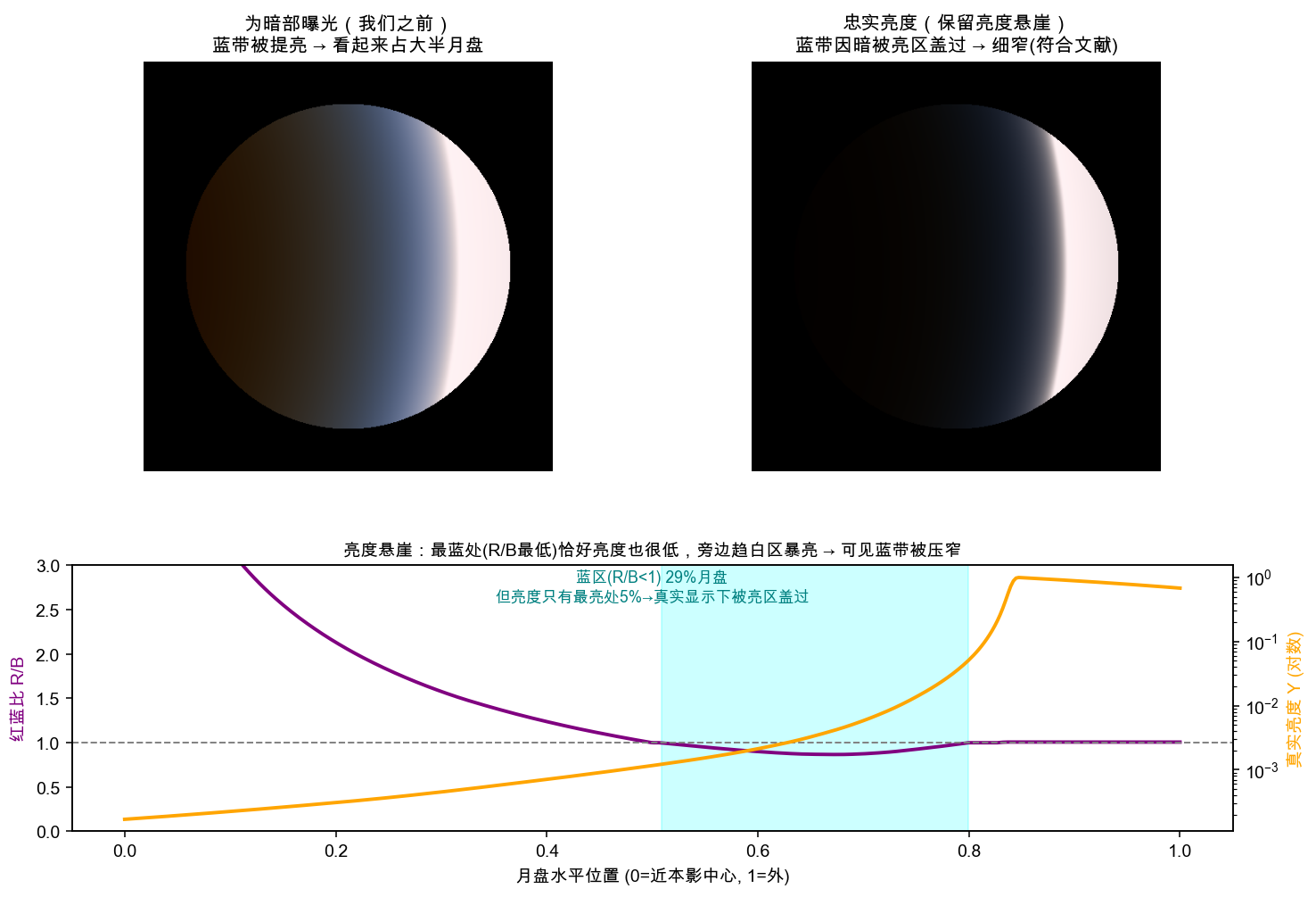
Figure 7: Brightness cliff — the bluest region is also the darkest, overshadowed by the bright white zone next to it, leaving only a thin band
Why does the turquoise band disappear at deepest totality? During deep totality the moon sits at the center of the umbra. The sunlight reaching it grazes at very low height; Rayleigh scattering scatters away blue light and leaves only red — the blood moon is reddest and darkest. Cyan appears when grazing height rises into the stratosphere — where Rayleigh scattering becomes secondary and ozone Chappuis absorption dominates, eating orange-red and leaving blue-green. But the stratosphere corresponds to the edge of the umbra, not the center. So the turquoise band is visible only when the moon moves toward the umbra edge and the brightness cliff begins to appear. At the deepest center of totality, the entire disk sits in Rayleigh's red zone; ozone's cyan never gets a stage.
Why Brute Force Works Now
Stepping back, I want to say something more general.
In scientific computing of this kind, approximation used to be a virtue. Supercomputer time was billed by the hour; PhDs who wrote programs had their skill points in physical intuition rather than software engineering; trading physical approximation for less and faster computation was rational. But that cost structure has inverted in the AI era. AI knows both physics and programming; deriving refraction formulas and writing GPU kernels takes minutes. A personal computer can scatter millions of rays; runtime is no longer the bottleneck. So "the art of approximation" turns from virtue into obstacle. Brute-force first-principles methods are now fast, accurate, and free of mutually masking free parameters — often the best approach.
That does not mean predecessors were wrong. They made optimal choices under their constraints. Mallama 2022's point-source assumption, closed-form refraction, and 1/r focusing were each reasonable approximations under a compute budget. Even García Muñoz and DLR's 2025 work, in an era when compute is no longer scarce, still chose semi-analytic methods for physical interpretability or real-time rendering. We should stay alert: the inertia of approximation does not disappear on its own. When constraints lift, skipping approximation is a very feasible alternative with fewer assumptions.
One clarification: we are not pushing brute-force computing as a universal doctrine. Human effort has limits; if you insist on fundamentalism and refuse all approximation, you will hit the compute wall again soon. The point is that this is not black and white. In 2026, with strong AI and strong machines, it is worth considering technical paths that skip approximation when doing scientific computing.
What a Lunar Eclipse Looks Like from the Moon
As in the previous article, once the simulation pipeline works, it can do many things real photography cannot — for example, explore by changing parameters.
We can compute the moon as seen from Earth; because our simulation is fully brute-force, we can swap the integration dimension and see the view from the moon. So we made a video showing Earth as seen from the moon. During a lunar eclipse, someone standing on the moon sees Earth completely blocking the Sun — a total solar eclipse on Earth. A ring of refracted light lights up the atmosphere on Earth's night side, color running from red on the inner edge through cyan to white on the outer edge — a sunset profile wrapped into a circle. As the moon moves out of the umbra, the Sun peeks from Earth's edge, one side of the atmospheric ring brightens, and finally becomes a diamond ring. The whole sequence is the same radiative transfer physics as before, just a different viewpoint.
Dual-view eclipse video: left — moon (moving out of umbra) | center — Earth panorama | right — atmospheric ring close-up
We also plotted a photometric curve: lunar surface brightness from the center of the umbra to full moon. The center is at −15 stops, then rises gradually to the brightness cliff at the umbra edge, then smoothly climbs to 0 stops at full moon. This curve is itself a diagnostic: if you see a jump somewhere, a piece of physics is missing. We once found a spurious jump leaving the umbra; tracing it down, direct sunlight in the penumbra was not modeled — light from the Sun peeking around Earth's edge. Ray trace that honestly and the jump disappears.
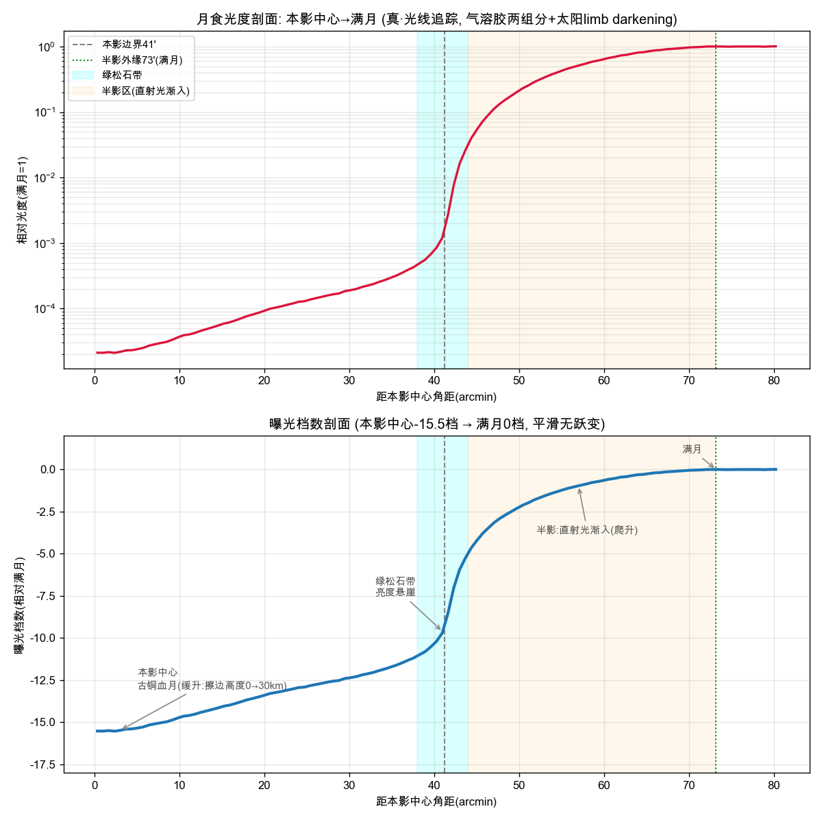
Figure 8: Photometric curve — umbra center at −15 stops to full moon at 0 stops, brightness cliff at 41 arcminutes
All results, code, and rendering scripts are on the project homepage. Feel free to play with them.
In Closing
We failed many times along the way, but each failure corrected an inaccurate understanding. The point-source approximation made us think the turquoise band would be strong; the focusing formula made the umbra center 250 times too bright. Every temptation to say "close enough" was answered by going back to physics and finding what was missing. Several times I saw the computed cyan too strong or the umbra too bright and wanted to tweak ozone concentration or add aerosols to darken it. Each time I held back. When the final pale cyan narrow band matched GOES-16 measurements and Shu 2024 remote sensing data point by point, I felt holding back was right.
The biggest takeaway from this project is that AI has lowered the barrier to first-principles physical simulation. People like me could not do this before because too many physical decision points required expert judgment. Now AI handles both physics and programming; the one judgment I need to make is: brute force, not clever approximation. That may be the most counterintuitive point about scientific computing in the AI era: the stronger AI gets, the more humans need the judgment not to take shortcuts.